Basic statistical concepts

Why statistics?

Kareem Carr via dddrew.com

Because they’re EVERYWHERE

We live in a world of randomness

Statistics help provide some strucure to the randomness

and allow us to extract useful information

Data are inherently random

If you collect a sample from a population

Then collect a second sample from the same population

They are very unlikely to be the same observations
(or measurements)

However some observations will occur more
frequently than others

So we can assume that we will observe an outcome a certain number of times

if an experiment (or analysis) is repeated
(even if we don’t actually repeat it)

This allows us to estimate parameters of a population

without tediously studying the whole population

and the more experiments we conduct

or the more data we collect

the closer we get to the true parameters
(as the number approaches infinity)

This is known as the Frequentist approach

And is the more common approach in most of science
(for now…)

A statistic is a single value describing a collection of observations (data from a sample)

Since these observations are not predictable, we can call them a random variable

A statistic is often assigned the generic symbol \(\text{T}\)

A random variable is assigned \(\text{X}\)

Statistics describing random variables, are themselves random variables (more later)

For example, measurements taken from a sheep’s astragalus

https://doi.org/10.1101/2022.12.24.521859

could be considered random variables

Let’s collect some measurements

sheep-data.csv

We can describe them in simpler terms
using descriptive statistics

We can calculate a central tendency of the data

The arithmetic mean (or ‘average’) of the GLl variable is: 30.34

It is calculated as

\[ \frac{1}{n} \Sigma_{i=1}^{n} GLl_i \]

Which is a fancy way of writing: all measurements of GLl added together (sum, or \(\Sigma\))

then divided by the number of measurements n, or sample size

Try it in R

sum(sheep_data$GLl) / length(sheep_data$GLl)

[1] 30.33866

mean(sheep_data$GLl)

[1] 30.33866

This is not very useful information in isolation

GIPHY

We need more context

A question we might ask is

how much do the data
vary around the mean?

We can calculate the difference between

the mean of our sample (\(\bar{x}\)) and each observation (\(x_i\))

and sum

\[ \sum(x_i - \bar{x}) \]

But that would essentially give us zero

because there is roughly an equal number of measurements below and above the mean

(hence it’s a measure of central tendency…)

so we square the result to remove negative values

\[ \sum_{i=1}^{n}(x_i - \bar{x})^2 \]

which gives us the
sum of squared differences

But

larger samples

will have

larger differences

making it difficult to compare different-sized samples

So we divide by sample size, n (minus 1), to standardise

\[ s^2 = \frac{\sum_{i=1}^{n}(x_i - \bar{x})^2}{n - 1} \]

and obtain the variance
\(s^2\)

Try it in R

sum((sheep_data$GLl - mean(sheep_data$GLl)) ** 2) / (length(sheep_data$GLl) - 1)

[1] 2.24968

var(sheep_data$GLl)

[1] 2.24968

Because we’re squaring the differences, the numbers can quickly get unruly

So we can take the square root of the variance

\[ s = \sqrt{s^2} = \sqrt{\frac{\sum_{i=1}^{n}(x_i - \bar{x})^2}{n - 1}} \]

to get the standard deviation
\(s\)

Try it in R

sqrt(var(sheep_data$GLl))

[1] 1.499893

var(sheep_data$GLl) ** (1/2)

[1] 1.499893

sd(sheep_data$GLl)

[1] 1.499893

Combined with the mean

standard deviation can say more about our data

But for the whole sample this is not very informative

We could calculate summary statistics across multiple groups

But how do we know if the groups differ (or not) in a meaningful way?

We could run some statistical test

but which one?

GIPHY

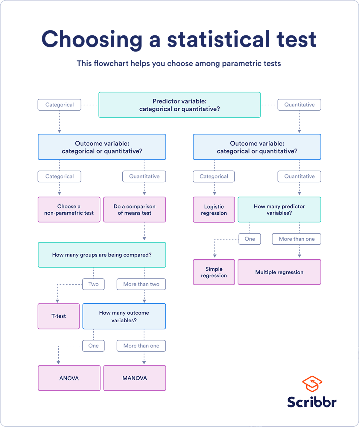
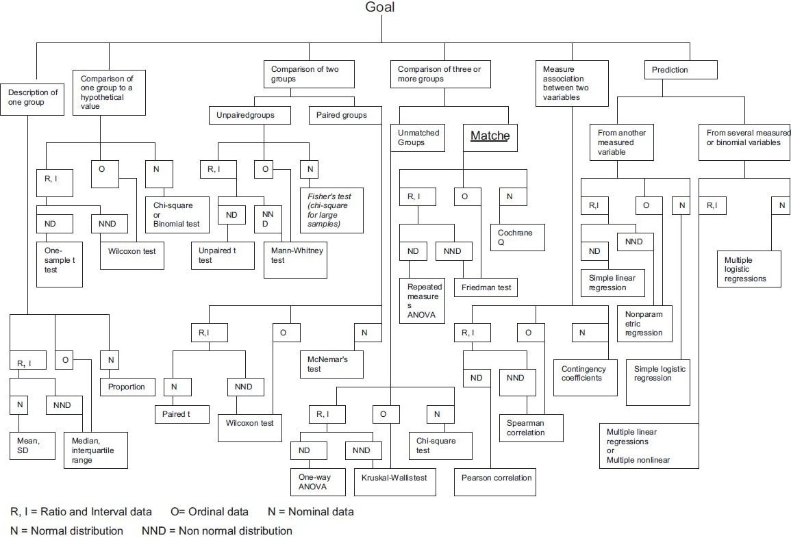
The correct answer: It depends…

Primarily it depends on what do your data look like?

R for Data Science

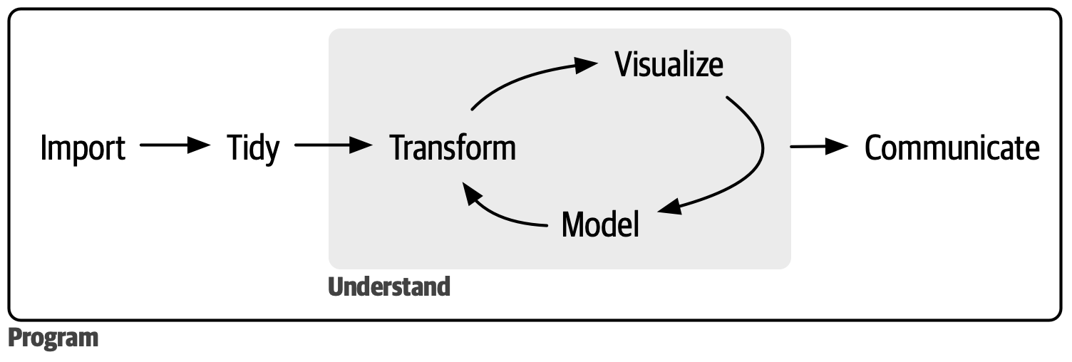
Descriptive statistics only get you so far…

z3tt/TidyTuesday

We need to explore the data